
ߞߐߕߐ߮:IQ curve.svg

ߣߌ߲߬ PNG ߢߊ߲ߞߊ߲߸ ߣߌ߲߬ SVG ߢߍߦߋߟߌ߸ ߞߐߕߐ߮: ߔߌߞߑߛߍߟ ߆߀߀ × ߄߈߀ ߢߊߓߐߟߌ ߟߎ߬ ߕߐ߬ߡߊ ߔߌߞߑߛߍߟ ߃߀߀ × ߂߄߀ | ߔߌߞߑߛߍߟ ߉߆߀ × ߇߆߈ | ߔߌߞߑߛߍߟ ߁,߂߈߀ × ߁,߀߂߄ | ߔߌߞߑߛߍߟ ߂,߅߆߀ × ߂,߀߄߈.
ߞߐߕߐ߮ ߓߊߛߎ߲ (SVG ߞߐߕߐ߮, ߕߐ߯ߦߊߟߌ ߆߀߀ × ߄߈߀ ߖߌ߬ߦߊ߬ߘߊ߲ߕߊ, ߞߐߕߐ߮ ߢߊ߲ߞߊ߲: ߉ KB)
ߟߊߘߛߏߣߍ߲
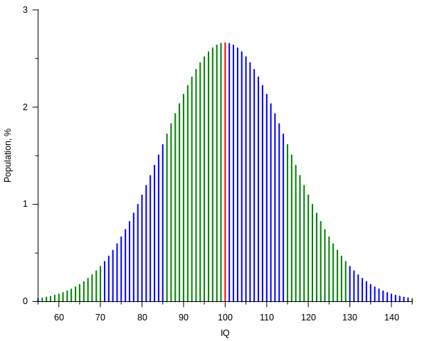
| ߕߐ߯ߟߊߘߏ߲ | Current IQ tests typically have standard scores such that the mean score is 100 with each standard deviation from the mean counting for 15 IQ points.[1] The plot shows, assuming that such scores have a normal distribution, the percentage of people getting a score versus the score itself, from 55 to 145 IQ, that is over a span of six standard deviations. Spans are represented with different colors for each standard deviation above or below the mean. The plot was created with the following gnuplot code: |
| SVG genesis | |
| Source code | Gnuplot codeset terminal svg name 'IQ_curve' size 600,480 font ',10' rounded
set output 'IQ_curve.svg'
mu = 100.0
sigma = 15.0
from = 55
to = 145
# Normal distribution:
# (continuos normalization approximation, good to ~10 digits in this case)
P(x) = exp(-(x - mu)**2 / (2 * sigma**2)) / (sqrt(2 * pi) * sigma) * 100
# By sigma intervals:
oddsi(x) = (int(abs(x - mu) / sigma) % 2) ^ (x < mu)
Pm(x) = (x == mu) ? P(x) : 1/0 # sample at mu
Po(x) = ( oddsi(x) && (x != mu)) ? P(x) : 1/0 # samples in odd sigma intervals
Pe(x) = (!oddsi(x) && (x != mu)) ? P(x) : 1/0 # samples in even sigma intervals
set key off
set border 3
set xlabel 'IQ'
set xtics 10 out nomirror
set mxtics 2
set ylabel 'Population, %'
set ytics 1 out nomirror
set mytics 2
set samples (to - from + 1)
set style function impulses
plot [x = from:to] \
Pm(x) lw 2, \
Po(x) lw 2, \
Pe(x) lw 2
|
| ߕߎ߬ߡߊ߬ߘߊ | |
| ߛߎ߲ | ߟߊ߫ ߓߊ߯ߙߊ ߟߋ߫ ߘߌ߫ |
| ߛߓߍߦߟߊ | Alessio Damato, Mikhail Ryazanov |
- ↑ Kaufman, A.S. (߂߀߀߉) IQ Testing 101, New York (NY): Springer Publishing, pp. 104−109 ISBN: 978-0-8261-0629-2.
ߟߊ߬ߘߌ߬ߢߍ߬ߟߌ ߦߴߌ ߘߐ߫
I, the copyright holder of this work, hereby publish it under the following licenses:

|
ߓߊߓߌߟߊߟߌ ߟߊߘߌ߬ߢߍ߬ ߣߍ߲߫߸ ߞߵߊ߬ ߘߐߕߟߊ߫ ߊ߬ ߣߌ߫/ߥߟߊ߫ ߞߊ߬ ߘߐ߬ߛߙߋ ߣߌ߲߬ ߡߊߦߟߍ߬ߡߊ߲߫ ߛߙߊߕߌ ߣߌ߲߬ ߠߊ߫ GNU Free Documentation License, ߡߊ߬ߦߟߍ߬ߡߊ߲߬ߣߠߌ߲ ߁.߂ ߥߟߊ߫ ߡߊ߬ߦߟߍ߬ߡߊ߲߬ߠߌ߲ ߜߘߍ ߛߎ߯-ߎ߯-ߛߎ߫ ߟߊߥߊ߲߬ߞߊ߫ ߣߍ߲߫ Free Software Foundation; ߓߟߏ߫, ߕߍߕߍ߯ ߞߕߐߡߊߛߊ߬ߦߌ߲߬ߣߍ߲ ߝߋ߲߫ ߕߍ߫߸ ߊ߬ ߞߣߐߟߊ ߥߣߊ߬ߙߌ߬ ߛߓߍߟߌ߫ ߕߍ߫߸ ߊ߬ ߣߌ߫ ߞߐߞߊ߲߫ ߥߣߊߙߌ ߛߓߍߟߌ߫ ߕߍ߫.ߊ߬ ߓߊߞߎߘߊ ߕߌ߰ߦߊ ߟߊߘߏ߲߬ߣߍ߲߬ ߦߋ߫ ߕߍߕߍ߮ ߣߌ߲߬ ߠߋ ߘߐ߫߸ ߞߴߊ߬ ߕߐ߯ߟߊ߫ ߞߏ߫ GNU Free Documentation License. |
| ߞߐߕߐ߮ ߣߌ߲߬ ߦߋ߫ ߞߍߦߙߐ ߣߌ߲߬ ߠߎ߬ Creative Commons Attribution-Share Alike 3.0 Unported ߟߊ߫ ߘߌ߬ߢߍ ߟߋ߬ ߘߐ߫ | ||
same or compatible license ߊ߬ ߛߎ߲ ߘߌ߫. | ||
| This licensing tag was added to this file as part of the GFDL licensing update. |
This file is licensed under the Creative Commons Attribution-Share Alike 2.5 Generic, 2.0 Generic and 1.0 Generic license.
- ߌ ߞߊ߲ߠߊߓߌ߬ߟߊ߬ߣߍ߲߫
- ߞߵߊ߬ ߟߊߖߍ߲ߛߍ߲߫ – ߞߊ߬ ߓߊ߯ߙߊ ߓߊߞߎߘߦߊ߫߸ ߞߴߊ߬ ߘߐߝߘߊ߫߸ ߊ߬ ߣߌ߫ ߞߵߊ߬ ߟߊߕߊ߬ߡߌ߲߬
- ߞߵߊ߬ ߢߣߊߓߊ߬ߛߊ߲߬ ߕߎ߲߯ – ߞߊ߬ ߓߊ߯ߙߊ ߟߊߘߏ߲߬
- ߓߍ߲߬ߒߡߊ߬ߞߊ߲߫ ߣߊ߬ߕߐ ߢߌ߲߬ ߠߎ߬ ߟߊ߫:
- ߘߎ߲߬ߘߎ߬ߡߊ߬ߦߊ – ߌ ߦߋ߫ ߞߍߕߊ ߓߍ߲߬ߣߍ߲ ߠߊߘߏ߲߬߸ ߞߊ߬ ߟߊ߬ߘߌ߬ߢߍ߬ߟߌ ߛߘߌ߬ߜߋ߲ ߘߏ߫ ߡߊߛߐ߫߸ ߊ߬ ߣߌ߫ ߞߊ߬ ߞߐ߯ߙߍߦߊ߫ ߣߌ߫ ߡߊ߬ߦߟߍ߬ߡߊ߲߬ߠߌ߲ ߞߍߣߍ߲߫ ߞߍ߫ ߘߊ߫. ߌ ߦߴߏ߬ ߞߍ߫ ߞߍߢߊ߫ ߟߊߘߌ߬ߢߍ߬ߣߍ߲ ߓߍ߯ ߡߊ߬߸ ߞߏ߬ߣߌ߲߬ ߢߊ ߓߍ߯ ߡߊ߬ ߞߏ߫ ߕߍ߫ ߘߋ߬߸ ߡߍ߲ ߘߌ߫ ߛߋ߫ ߟߊ߬ߘߌ߬ߢߍ߬ߟߊ ߘߐߛߎ߫ ߟߴߌ ߞߊ߲ߛߏ߲߫ ߡߊ߬߸ ߥߟߊ߫ ߌ ߟߊ߫ ߟߊ߬ߓߊ߰ߙߊߟߊ.
- ߘߍ߬ߒ߬ߡߊ߬ ߝߋ߲ – ߣߴߌ ߞߵߊ߬ ߡߊߦߟߍ߬ߡߊ߲߫߸ ߖߙߎߡߎ߲ ߦߟߍ߬ߡߊ߲߫߸ ߥߟߊ߫ ߞߵߊ߬ ߓߊ߯ߙߊ ߓߐ߬ߓߐ ߣߌ߲߬ ߞߊ߲߬߸ ߌ ߞߍߕߐ߫ ߦߋ߫ ߞߐߖߋߓߌ߫ ߞߋߟߋ߲߫ ߠߋ߬ ߘߐߝߘߊ߫ ߟߊ߫ ߥߟߊ߫ ߌ ߟߊ߫ ߡߊ߬ߜߍ߲ ߞߍ߫ ߕߐ߫ ߦߋ߫
ߌ ߘߌ߫ ߛߴߌ ߘߌߦߊߣߊ߲߫ ߕߦߊ ߛߎߥߊ߲ߘߌ߫ ߟߊ߫
ߞߐߕߐ߮ ߟߊ߫ ߘߐ߬ߝߐ
ߕߎ߬ߡߊ߬ߘߊ/ߕߎ߬ߡߊ ߛߐ߲߬ߞߌ߲߬ ߓߊ߫߸ ߞߊ߬ ߕߎ߬ߡߊ߬ߘߊ ߞߐߕߐ߮ ߟߎ߬ ߦߋ߫.
| ߕߎ߬ߡߊ߬ߘߊ/ߕߎ߬ߡߊ߬ߟߊ߲ | ߞߝߊ߬ߟߋ߲ߛߋ߲ | ߛߎߡߊ߲ߘߐ | ߟߊ߬ߓߊ߰ߙߊ߬ߟߊ | ߞߊ߲߬ߝߐߟߌ | |
|---|---|---|---|---|---|
| ߞߍߛߊ߲ߞߏ | ߂߃:߁߁, ߂߆ ߣߍߣߍߓߊ ߂߀߂߀ | | ߆߀߀ × ߄߈߀ (߉ KB) | Paranaja | Reverted to version as of 21:27, 2 November 2012 (UTC) |
| ߂߁:߂߇, ߂ ߣߍߣߍߓߊ ߂߀߁߂ |  | ߆߀߀ × ߄߈߀ (߉ KB) | Mikhail Ryazanov | IQ values are now integers; gnuplot-only approach | |
| ߀߉:߂߀, ߆ ߞߏߟߌ߲ߞߏߟߌ߲ ߂߀߀߆ |  | ߆߀߀ × ߄߈߀ (߁߂ KB) | Alejo2083 | {{Information |Description= The IQ test is made so that most of the people will score 100 and the distribution will have the shape of a Gaussian function, with a standard deviation of 15. The plot shows the percentage of people getting a score versus the |
ߞߐߕߐ߮ ߟߊߓߊ߯ߙߊߟߌ
ߞߐߜߍ߫ ߛߌ߫ ߡߊ߫ ߞߐߕߐ߮ ߣߌ߲߬ ߠߊߓߊ߯ߙߊ߫ ߡߎߣߎ߲߬
ߞߐߕߐ߮ ߟߊߓߊ߯ߙߊߟߌ߫ ߞߙߎߞߙߍ
ߥߞߌ߫ ߕߐ߭ ߢߌ߲߬ ߠߎ߬ ߦߋ߫ ߞߐߕߐ߮ ߣߌ߲߬ ߠߊߓߊ߯ߙߊ߫ ߟߊ߫:
- ߊ߬ ߟߊߓߊ߯ߙߊ߫ ar.wikipedia.org ߘߐ߫
- ߊ߬ ߟߊߓߊ߯ߙߊ߫ ast.wikipedia.org ߘߐ߫
- ߊ߬ ߟߊߓߊ߯ߙߊ߫ az.wikipedia.org ߘߐ߫
- ߊ߬ ߟߊߓߊ߯ߙߊ߫ ba.wikipedia.org ߘߐ߫
- ߊ߬ ߟߊߓߊ߯ߙߊ߫ be-tarask.wikipedia.org ߘߐ߫
- ߊ߬ ߟߊߓߊ߯ߙߊ߫ be.wikipedia.org ߘߐ߫
- ߊ߬ ߟߊߓߊ߯ߙߊ߫ ca.wikipedia.org ߘߐ߫
- ߊ߬ ߟߊߓߊ߯ߙߊ߫ cs.wikipedia.org ߘߐ߫
- ߊ߬ ߟߊߓߊ߯ߙߊ߫ da.wikipedia.org ߘߐ߫
- ߊ߬ ߟߊߓߊ߯ߙߊ߫ de.wikipedia.org ߘߐ߫
- Intelligenzquotient
- Normwert
- Wikipedia:WikiProjekt Psychologie/Archiv
- Benutzer:SonniWP/Hochbegabung
- Kritik am Intelligenzbegriff
- The Bell Curve
- Benutzer:Rainbowfish/Bilder
- Quantitative Psychologie
- Intelligenzprofil
- Benutzer:LauM Architektur/Babel
- Benutzer:LauM Architektur/Babel/Überdurchschnittlicher IQ
- ߊ߬ ߟߊߓߊ߯ߙߊ߫ de.wikibooks.org ߘߐ߫
- Elementarwissen medizinische Psychologie und medizinische Soziologie: Theoretisch-psychologische Grundlagen
- Elementarwissen medizinische Psychologie und medizinische Soziologie/ Druckversion
- Elementarwissen medizinische Psychologie und medizinische Soziologie/ Test
- Benutzer:OnkelDagobert:Wikilinks:Psychologie
- ߊ߬ ߟߊߓߊ߯ߙߊ߫ de.wikiversity.org ߘߐ߫
- ߊ߬ ߟߊߓߊ߯ߙߊ߫ en.wikipedia.org ߘߐ߫
- User:Michael Hardy
- User:Robinh
- User:Itsnotvalid
- User:M.e
- User:Quandaryus
- User:Astronouth7303
- User:Mattman723
- User:Iothiania
- User:Octalc0de
- Portal:Mathematics/Featured picture archive
- User:Dirknachbar
- User talk:BlaiseFEgan
- User:Albatross2147
- User:Klortho
- User:Kvasir
- User:Spellcheck
- User:Heptadecagram
- User:Patrick1982
- User:NeonMerlin/boxes
- User:Cswrye
ߞߐߕߐ߮ ߣߌ߲߬ more global usage ߦߋߟߌ.